Geographical Mapping of Denmark in SAS

Introduction

Creating accurate maps of countries and their states or municipalities can be an interesting way to showcase data across a geospatial dimension. Nearly everything desired in this context can be achieved using SAS’s g-functions. A heatmap can effectively display diversity across regions, and additional functions can further enhance the program and its outputs.

Below is a section where a heatmap of Denmark and its municipalities is created in SAS. This program can be modified to feature other countries and regions. Several interesting functions have been added to the program, allowing for customization and enhancement:

Automatically generated intervals for the heatmap (based on Nelder’s algorithm), highlighting regional diversity.

Conversion of input data values to numerical format if they are character values (convertible ones like “0.53”).
An option to apply formatting to values as desired (including setting intervals for displayed values).
Distinct color schemes for categorical and continuous variables.
A zoomed inset for small or remote regions.
Exporting the output image as PDF or PNG.
Saving the map function as a permanent macro using mstored, enabling easy integration into other programs.

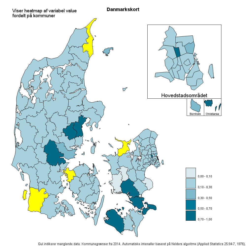
The map functions result in a visualization like this:

	%map(
		Dataset = 			/* Mandatory. Dataset. */
		,Var =				/* Mandatory. Variable to plot. */
		,output_path = 			/* Optional. Output path if PDF is desired. */
		,ID =				/* Optional. ID code, e.g. state name. Standard: ID */ 
		,discrete_or_cat =      	/* Optional. Discrete or categorical variable. Standard: Discrete */
		,nlevels =			/* Optional. Number of intervals. Standard: 5. Standard: 5 */
		,format = 			/* Optional. Display value format. Standard: commax10.2. */
		,miss_color			/* Optional. Missing data color. Standard: yellow */
				)

The finished product could look something like this (using automatically generated intervals):

Construction

Only the essential parts are included; message me if you’re interested in more details :)

Using the maps already integrated in SAS, the different parts of the map need to be allocated to different datasets to display them in various positions. This involves creating different datasets based on the ID (municipal code in this example):

/* Mainland Danmark */
data dk_map;
	set mapsgfk.denmark;
	&ID. = substr(ID,4,3)*1;
	if &ID. in (400,411) then delete;
run;

/* Bornholm */
data dk_map_born;
	set mapsgfk.denmark;
	&ID. = substr(ID,4,3)*1;
	if &ID. not in (400) then delete;
run;

/* Christiansø */
data dk_map_chris_oe;
	set mapsgfk.denmark;
	&ID. = substr(ID,4,3)*1;
	if &ID. not in (411) then delete;
run;

/* København */
data dk_map_kbh;
	set mapsgfk.denmark;
	&ID. = substr(ID,4,3)*1;
	if &ID. not in (
						 101
						,147
						,151
						,153
						,155
						,157
						,159
						,161
						,163
						,165
						,167
						,173
						,175
						,183
						,185
						,187
						,190
								) then delete;
run;

First, import the data you wish to display on the map. If a variable is a character and can be converted to a numerical value, include a conversion step:

data &Dataset._map_temp;
	set &Dataset.;
	if &var. = . then delete;
	vartype = VTYPE(&ID.);
	if vartype = "C" then do;
		&ID._ = &ID.*1;
		drop &ID.;
		rename &ID._ = &ID.;
	end;
	if vartype = "N" then do;
		&ID._ = &ID.;
		drop &ID.;
		rename &ID._ = &ID.;
	end;
	format &ID._;
run;

Both the map data and the data to be displayed are now imported. Use the proc gmap procedure to display the maps. Create all the maps from the datasets we previously prepared, so they can eventually be combined into the same image. An example of the map creation process might look like this:

/* Genererer kort af Mainland Danmark */
goptions xpixels=1000 ypixels=1000;
proc gmap
	map=dk_map
    data=&Dataset._map_temp all;
	format &var. &format.;
  	id &ID.;
   	choro &var. /
		legend=legend1
		coutline = black
		cdefault = &miss_farve.
		levels = &nlevels.
		midpoints = OLD RANGE
		name = "DK"
;
	title ls=1.5 "Danmarkskort";
		title2 angle=-90 height=25pct ' '; /* Dummy titel der skubber kortet til siden */

	note 
		move=(5,95)pct
		justify = left 
		height=1 
		"Viser heatmap af variabel &var."
	j=l
		move=(5,93)pct
		justify = left 
		height=1
		"fordelt på kommuner";
run;
title;
title2;
footnote;

and

/* Genererer kort af Bornholm */
footnote1 h=15pct "Bornholm";

goptions xpixels=100 ypixels=100;
proc gmap map=dk_map_born data=testdata all;
format &var. &format.;
id &id.; 
choro &var. / 
		nolegend
		coutline = black
		cdefault = &miss_farve.
		levels = &nlevels.
		midpoints = OLD RANGE
		name='born'
		;
run;
footnote;

Repeat this process for all intended map parts.

Name these maps correspondingly, e.g., ‘born’ for Bornholm. Use the proc greplay procedure to layer all these maps on top of each other, as follows:

/* Kører greplay */
proc greplay tc=tempcat nofs igout=work.gseg;
  tdef crmap des='crmap'
   1/llx = 0   		lly = 0
     ulx = 0   		uly = 100
     urx = 100  	ury = 100
     lrx = 100  	lry = 0

   2/llx = 76  		lly = 53 
     ulx = 76	  	uly = 60
     urx = 83 	 	ury = 60
     lrx = 83	  	lry = 53
	 color=black

   3/llx = 83  		lly = 53
     ulx = 83	  	uly = 60
     urx = 90	  	ury = 60
     lrx = 90	  	lry = 53
	 color=black

   4/llx = 60  		lly = 60 
     ulx = 60	  	uly = 90
     urx = 90	  	ury = 90
     lrx = 90	  	lry = 60
	 color=black

;
template = crmap;
treplay
 1:DK
 2:born
 3:chris_oe
 4:kbh
 ;
run;

This approach will compile the maps into a single image. Ensure the sizes of the x and y coordinates match the dimensions of the map image set by commands like goptions xpixels=100 ypixels=100;.

This is the main structure of the program. Additional features can be added to incorporate the functions mentioned in the introduction.

Oliver Weeks

Introduction

Construction